Back in the summer of 2020, I stumbled across a YouTube video featuring computer science professor presenting his algorithm for solving Sudoku puzzles. At the end of the video, he challenges viewers to tackle a much more difficult puzzle: the sliding-block puzzle, Klotski. This challenge set me on a years-long journey of creating and optimizing Klotski-solving algorithms in various languages, culminating in a web app that utilizes the most recent iteration of the algorithm. Here's how I cracked Klotski.
Understanding the Game
First, it's important to introduce the game of Klotski. Klotski puzzles traditionally take place on a grid with five rows and four columns. There are four block variants used in these puzzles, and some arrangements of these blocks is placed onto the grid, leaving exactly two empty cells.
Every puzzle must contain exactly one big block, which is two cells tall and two cells wide. The goal of the game is to move this block into the winning position: the bottom middle of the grid.
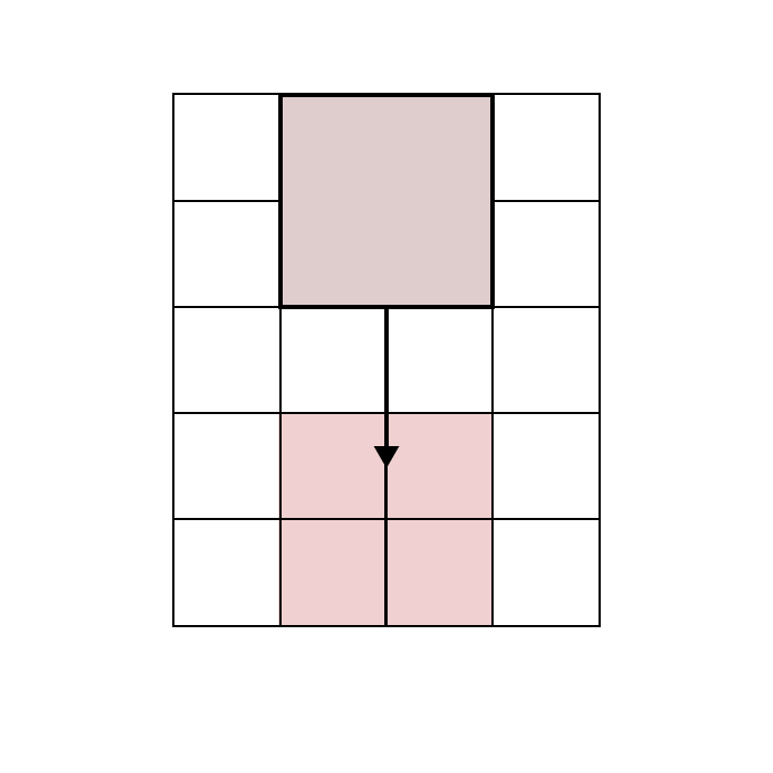
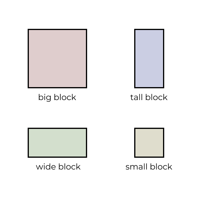
In between the big block and the winning position, the grid will contain some number of the three remaining block types:
- The tall block, which is two cells tall and one cell wide
- The wide block, which is one cell tall and two cells wide
- The small block, which is one cell tall and one cell wide
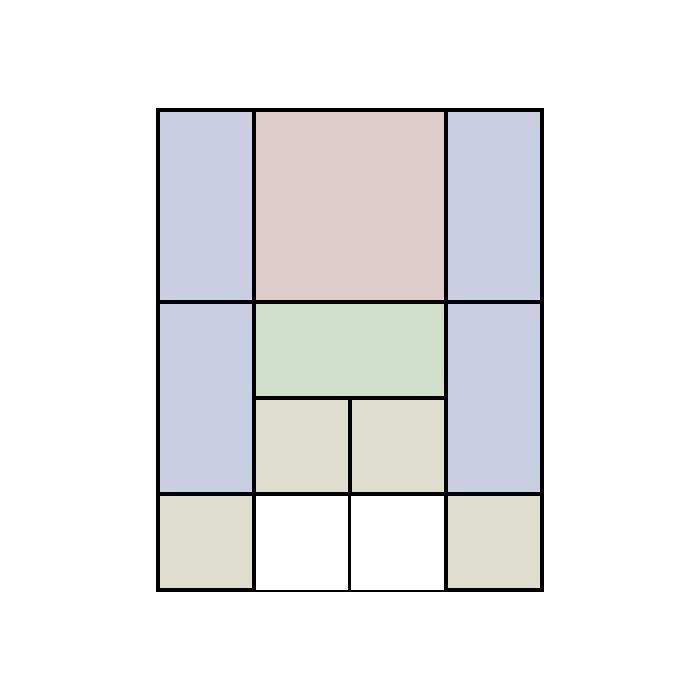
Once the board is set up according to these rules, the player must slide individual blocks to allow the big block passage toward the bottom of the grid. Each move consists of sliding a block one or two spaces.
The Human Approach
After understanding the game, anyone can go about solving a Klotski puzzle, albeit with a lot of trial and error. Sometimes the big block gets stuck and can no longer move downward, forcing you to backtrack to a point in time where a valid path seemed to still exist. Once you've solve a puzzle, however, a question will emerge. Can this puzzle be solve in fewer moves? I personally have spent a substantial amount of time replaying these puzzles, changing a move here and there in hopes of reducing the final move count. Can we write an algorithm that always finds the solution with the fewest possible moves?
Representing the Problem as a Tree
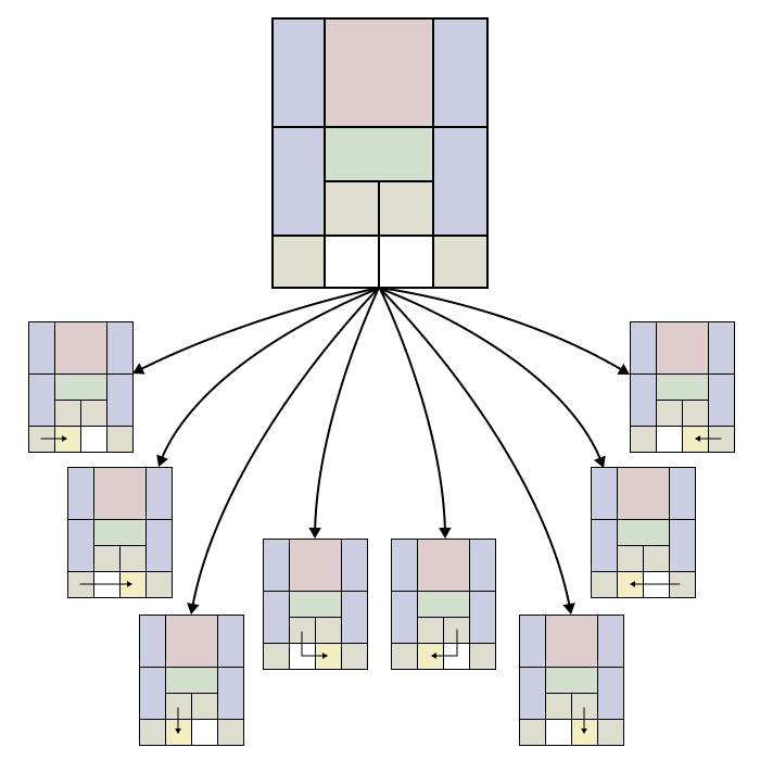
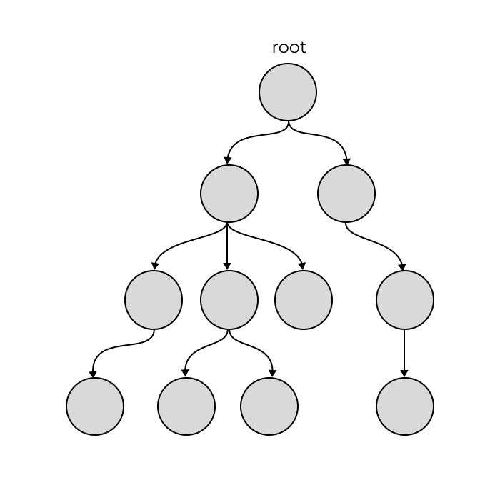
How can we go about automating this process? Interestingly, the solution mimics a human's process of trial and error but much more efficiently and exhaustively. Let's consider our initial board as the root of a decision tree. Our board will have some number of possible next moves which will correspond to the available decisions. The boards that result from these moves will make up the next level of our decision tree.
Finding an Optimal Solution
This first set of children represents all possible boards resulting from a single move. Similarly, each level of our tree contains all boards resulting from moves on the start board. Because we explore every possible move, then if our board is solvable, at some level we will first encounter a solved board. Since this is the first time we have encountered a solved board, we know it must be an optimal solution. If not, we would have seen a solved board in one of the previous levels. We also know that the minimum number of moves required to solve our board is .
Once we have found our first solved board, we can stop, knowing we are at the end of an optimal decision path. To retrieve the moves that comprise this path, we trace our steps back, traversing the decision tree upwards from the solved board to the initial board. This path represents our optimal solution in reverse.
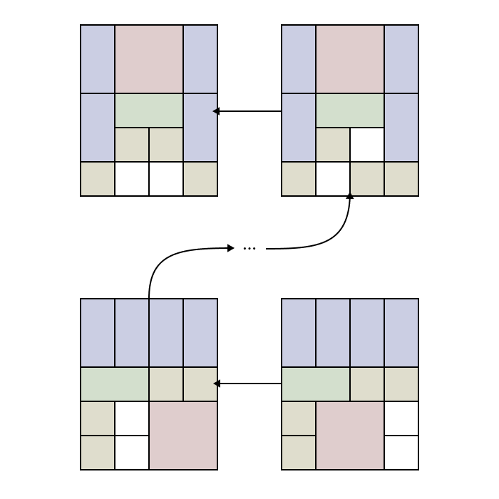
While it makes sense that exploring every possible move eventually leads to an optimal solution, a more interesting question arises: can we reduce the number of moves we explore and still reach the solution?
Avoiding Non-Progressive Moves
One of the first things we will notice as we examine the levels of our decision tree is the significant repetition of board configurations. For instance, if a move is valid for a given board, then in the resulting board, the opposite move will also be valid. This is a redundant move and should be avoided. One approach to address this would be to have our algorithm remember the previous move and exclude its opposite from the set of valid next moves. However, this approach doesn't solve the case where a sequence of moves, though not immediately reversing each other, ultimately returns us to where we started. How can we overcome these non-progressive moves?
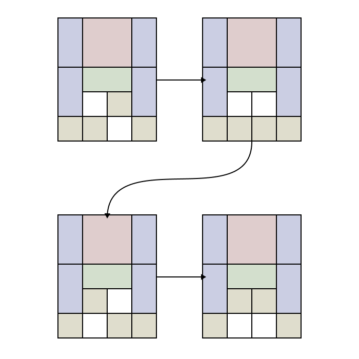
What if we save every board configuration we encounter and only consider moves valid if they generate new configurations? Could this greedy choice be effective? This approach would only be invalid if there exists a case where two sequences of moves lead to the same board configuration and only the longer of the two leads to a solved board. Why would this invalidate our approach? If this were the case, then the shorter sequence of moves will reach the board configuration first, thereby invalidating the longer sequence and missing a potential optimal solution.
Could this scenario ever occur? If a shorter set of moves reaches a particular board configuration and doesn’t lead to a solution, then the longer set, which only adds redundant moves, will also not lead to a solution. Therefore, by ensuring that each move generates a unique board configuration, we eliminate non-progressive sequences and efficiently guide the algorithm toward the optimal solution. It turns out that with this minor adjustment, we can solve any Klotski puzzle quite quickly.
The Breadth-first Search Algorithm
It turns out that the high-level approach we have been describing is an application of a well-known algorithm called Breadth-first Search (BFS). BFS is a graph traversal algorithm that has many real-world applications, from web crawling to social network analysis to chess engines. In the case of our Klotski solver, BFS is particularly suitable because it can find the shortest path in an unweighted graph, meaning a graph where each edge—or in our case each move—has the same weight.
BFS can be run on any graph, but in our case, we are running it on a specific type of graph called a tree. Trees are a unique subset of graphs where each node in the structure has exactly one parent but can have multiple children. The only exception is the root node, which has no parent.
In BFS, we use a data structure called a queue to store the current level of the tree. Queues are a collection of elements that allow removal from the front and addition at the back. Like any queue that enforces rules against cutting, the first entrant into the queue should also be the first to leave. This is why queues are referred to as first-in-first-out (FIFO) data structures. Adding to the end of a queue is traditionally done with a method called enqueue, and removal from the front of a queue with a method called dequeue.
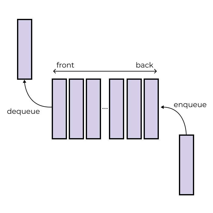
The queue will initially contain just the starting board. Once we have processed this board, the queue will contain all of the unique boards that result from a single move. After those boards have been processed, the queue will contain all unique boards that result from another move. This process will repeat itself until we have either reached a solved board or all possibilities are exhausted, meaning there is no solution.
To keep track of the boards we have seen, we need to use a data structure called a hash map. Hash maps store sets of key-value pairs and allow us to efficiently look up the value associated with a given key.
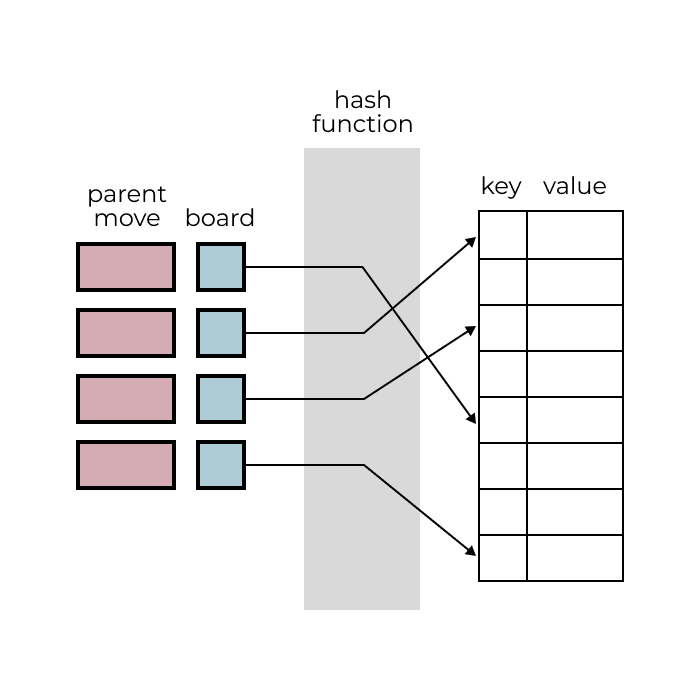
In our case, we'll use the board as our key and the move that led to the creation of the board—its parent move—as our value. Technically we need to use a hash function to convert the board into a hashable representation that the hash map can understand, but we will leave this out for simplicity. This hash map will allow us to efficiently check if a board has been seen and also retrieve the move that led to it.
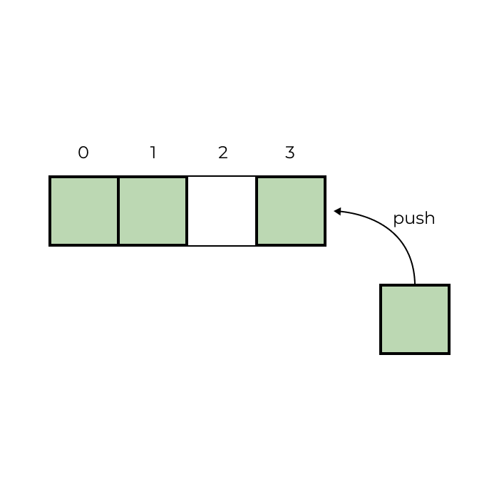
The final data structure that we is a dynamic collection of elements, often referred to as a vector, list, or dynamic array. Vectors are a resizable collections of elements. Items are traditionally added to the end of a vector with a method called push. The final result of our solver will be the vector of moves that make up our solution.
With this introduction to BFS and the key data structures involved, we're now ready to dive into the implementation of our solver.
Solver Implementation
Our solver will start by setting up our data structures. We will create a queue containing whose only node is our start board and a hash map containing one pair with our start board as the key and null as the value. This is because our start board has no parent move.
While our queue has contents, we will perform the following steps. If we reach a point where the queue is empty, then the board has no solution and we can return.
- Calculate the size of the queue, , and repeat the following times to process the current level:
- Dequeue a node and check to see if it is solved
- If it is solved, we are done
- If it is not solved, obtain its valid next moves and, for each move, do the following:
- Execute the current move on the board and check to see if the resulting board has been seen before in our hash map
- If it has been seen, we will skip it, so undo the current move on the board and continue to the next move
- If it has not been seen
- Enqueue a copy of the current board
- Update the hash map with a new pair containing the updated board as the key and the current move as the value
- Undo the current move on the board and continue to the next move
- Execute the current move on the board and check to see if the resulting board has been seen before in our hash map
- Dequeue a node and check to see if it is solved
The final step once a solved board is found is to create our moves vector. We can do so as follows.
Set up an empty vector called moves. Start with our solved board as the current board, and repeat the following steps until we are done.
- Lookup the current board's parent move in the hash map
- If no parent move exists, we are at the start board
- Reverse our moves vector and return it
- If a parent move does exist
- Push it to our moves vector
- Set the current board to its parent by undoing the parent move and continue
- If no parent move exists, we are at the start board
That's it! Here is some Python pseudocode to better visualize the algorithm.
Pythondef klotski_solver(start_board):
	# Initialize the queue and hash map
	queue = Queue()
	queue.enqueue(start_board)

	hash_map = HashMap()
	hash_map[start_board] = None

	# Process the queue, level-by-level, until it is empty
	while len(queue) > 0:
		n = queue.size()

		# Process each board in the current level
		do n times:
			current_board = queue.peek()
			queue.dequeue()

			# Check if the board is solved
			if is_solved(current_board):
				# If so, recreate the moves from the solved board to the start board
				parent_move = hash_map[current_board]
				moves = Vector()

				while parent_move is not None:
					moves.push(parent_move)

					# Undo the parent move, turning the current board into its parent
					make_move(
						current_board,
						get_reverse_move
					)

					parent_move = hash_map[current_board]

				# Return success with the reversed moves
				return Success(moves.reverse())

			# Find and process the valid next moves of the unsolved board
			next_moves = get_valid_moves(current_board)

			for move in next_moves:
				# Execute the current move on the board
				make_move(current_board, move)

				# Check if the board has not been seen
				if hash_map[current_board] is None:
					# If so, update the hash map and add the child board to the queue
					hash_map[current_board] = move
					queue.enqueue(clone(current_board))

				# Undo the previous move on the board
				make_move(
					current_board,
					get_reverse_move(move)
				)

	# The board is unsolvable, return failure
	return Failure()
Key Omissions and their Implications
I have purposely left out some important details. Firstly, I have not described the structure of the Klotski board: the grid, its blocks, or the moves that make up our solution. These type definitions are a complex and interesting topic in their own right. The focus of this post is to take all of that as given and explain the core features of the algorithm used to solve one of these puzzles.
Because the structure of the board components is not defined, I have also omitted the implementation of the following crucial functions. These functions will vary significantly based on the specific design decisions made regarding the board's components.
clone(board): Creates a copy of a boardis_solved(board): Checks whether the board is solvedget_valid_moves(board): Returns the set of valid moves for the boardmake_move(board, move): Executes a move on a boardget_reverse_move(move): Calculates the reverse of a move
Despite these omissions, there are still optimizations that can be made to our algorithm. These optimizations make use of more advanced topics in computer science, but can serve as interesting topics of further study for interested readers.
Optimizations
Space Optimization
Without going into detail about the structural representations of the puzzle's components, it is difficult to discuss space savings. These decisions will be the most crucial in determining the spatial efficiency of our algorithm. As far as our algorithm is concerned, our efforts to improve its runtime will bear more fruit.
Time Optimization
There are many ways we could attempt to optimize the runtime of our algorithm. I will go over a few of them briefly.
Returning a Linked List of Moves
One small optimization that we can make has to do with our process of reconstructing the final set of moves. In our example, we push new parent moves to the end of a vector and then reverse it. We do this because adding elements to the front of a vector is expensive. Every time we add an element to the front of a vector, we need to move every other element over one position. This takes time. Because of this we are happy to create the vector in our bottom-up traversal and then reverse it at the end. But what if there were another way?
With a linked list data structure, we can efficiently add elements to the front. Linked lists are exactly what they sound like, a list made up of linked elements. When we add another element to the front of a linked list, we are not adding it to the first position and then shuffling the locations of its other elements. We are linking our element to the head of the list, turning our element into the new head of the list.
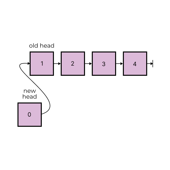
By replacing our moves vector with a linked list, we can add moves to the front and then return the final list as our answer, allowing us to avoid any reversal. However, since these sequences rarely contain much more than 100 moves, this is a small optimization.
Prioritizing Moves
Another more complicated optimization involves ranking the available moves on a board. We will first need to come up with some ranking function, commonly called a heuristic. This function will take a child board and tell us how close it is to being solved. The way we define this optimization is up to us. We may for instance rank a board based on how far away the big block is from the winning area or how many blocks stand in its way.
Once we have a heuristic function, we can convert our queue into a data structure called a priority queue, which maintain an ordering of its elements based on their ranks. If we pick a good heuristic function, this will allow our algorithm to make informed decisions on which paths to take first.
Parallelism
Finally, one practical approach to take on modern computers is to spread the work across multiple processors. For every level of our tree, we can divide the nodes across some number of processors, which will each process their share of the nodes. This processor will work in parallel, reading from and writing to our algorithm's shared state, including our queue and hash map. Because of this, we need to make sure we are using versions of these data structures that allow for concurrency. This approach will significantly reduce our runtime if implemented correctly.
Conclusion
Creating a Klotski solver can be challenging, but the process of developing and refining my approach has been incredibly rewarding. This solver has become my go-to project whenever I learn a new language, and with each iteration, I continually discover new insights.
For readers interested in implementing their own solvers, a great next step is to consider the best ways to structure the components of a Klotski puzzle, including the grid, blocks, and moves. When designing these structures, it is crucial to think about the functions that will interact with them.
Additionally, for those eager to delve into more advanced topics in computer science, I recommend investigating the implementation of the data structures we've used. They are some of the most common data structures in computer science and learning their implementation is a great start for anyone interested in the field. Finally, the suggested optimizations to our algorithm, including developing a heuristic and parallelization, are also great albeit challenging concepts to explore next.
Thank you for joining me on this tour of Klotski solving. I hope this post inspires you to take on your own challenging projects and experience the satisfaction of solving complex problems through code.